One of the best way to get a physical understanding of the Van Hoof effect is to
proceed to the analysis of the differential curves of velocity, radius
separation and acceleration of the two elements as previously done
(see Paper I). Figure![]() shows these three curves for FeI-FeII
lines presented above. The stellar restframe velocity
shows these three curves for FeI-FeII
lines presented above. The stellar restframe velocity ![]() is given by
is given by
 |
(1) |
where ![]() is the heliocentric radial velocity, V* the
stellar restframe velocity and p the geometrical projection and
limb-darkening correction factor. The velocity difference
is the heliocentric radial velocity, V* the
stellar restframe velocity and p the geometrical projection and
limb-darkening correction factor. The velocity difference
 |
(2) |
does not depend on the estimated value of V*.
It is only affected by the accuracy of the laboratory wavelength of each
absorption line and by the adopted p-value.
Note that an error of 0.1Å on one wavelength introduces a velocity
shift of 0.6km/s. Thus we expect that the
![]() -curve can be more or less shifted from its real position
by less than 1km/s. Although we have taken a constant p-value equal to
1.36, this shift is probably phase dependent because p varies
during the pulsation (Sabbey et al. 1995).
-curve can be more or less shifted from its real position
by less than 1km/s. Although we have taken a constant p-value equal to
1.36, this shift is probably phase dependent because p varies
during the pulsation (Sabbey et al. 1995).
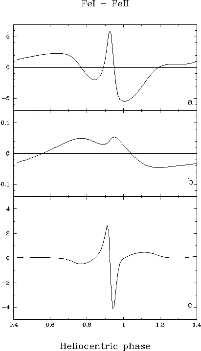 |
From pulsation phase ![]() (maximum radius) to
(maximum radius) to
![]() (middle of the contraction), FeI and FeII line forming
regions have the same variation of their acceleration (Fig.
(middle of the contraction), FeI and FeII line forming
regions have the same variation of their acceleration (Fig.![]() c).
They are not equal because the differential radius linearly
increases during this phase interval (Fig.
c).
They are not equal because the differential radius linearly
increases during this phase interval (Fig.![]() b).
If we accept, as shown by the Fokin's model, that the FeII line is formed
higher than the FeI line during the expansion, then the average distance
between these two regions reaches a value near to 0.05R
b).
If we accept, as shown by the Fokin's model, that the FeII line is formed
higher than the FeI line during the expansion, then the average distance
between these two regions reaches a value near to 0.05R![]() between phases 0.42 and 0.64 i.e., 50% of their maximum separation.
During this time, the differential radial velocity only increases by
1km/s. It can be surprising that the average separation between
FeI and FeII increase during the contraction. In fact, and as shown by
theoretical models (Fokin & Gillet 1997), the motion of atmospheric
layers already above the photosphere is extremely nonlinear for a star such
as RR Lyr. A series of rarefactions and compressions can occur at the same time
on the line of sight due to the complicated ballistic process.
between phases 0.42 and 0.64 i.e., 50% of their maximum separation.
During this time, the differential radial velocity only increases by
1km/s. It can be surprising that the average separation between
FeI and FeII increase during the contraction. In fact, and as shown by
theoretical models (Fokin & Gillet 1997), the motion of atmospheric
layers already above the photosphere is extremely nonlinear for a star such
as RR Lyr. A series of rarefactions and compressions can occur at the same time
on the line of sight due to the complicated ballistic process.
From ![]() , i.e., just before the photospheric minimum radius,
the differential acceleration of the Fe line forming regions begin to decrease
(up to 0.5 m/s2) because they penetrate more and more in
the dense photosphere, slowing down their free fall motion.
Because FeII is expected to be formed higher, the deceleration
is first stronger for FeI layers than for FeII ones.
This effect becomes visible near phase 0.77, because the differential
velocity and radius are decreasing (Figs.
, i.e., just before the photospheric minimum radius,
the differential acceleration of the Fe line forming regions begin to decrease
(up to 0.5 m/s2) because they penetrate more and more in
the dense photosphere, slowing down their free fall motion.
Because FeII is expected to be formed higher, the deceleration
is first stronger for FeI layers than for FeII ones.
This effect becomes visible near phase 0.77, because the differential
velocity and radius are decreasing (Figs.![]() a and b).
Until this phase, the FeI velocity was a little bit larger than
the FeII velocity. Both differential acceleration and radius reach
a maximum at phase 0.77 when the FeI velocity becomes smaller than
the FeII one and then begins to decrease. This is the consequence of
the progressive increase breaking induced by the dense atmosphere during the
contraction. All these effects occur during the secondary photospheric
acceleration centered at about phase 0.77 in our FeI and FeII
acceleration curves (not shown here). A stillstand is also visible
in the radial velocity curve at this phase (Paper II). Fokin &
Gillet (1997) showed that a shock wave (s3) produces at this time
an additional local compression of the atmospheric layers in which metallic
lines are formed. This shock was called the ``early shock'' by Hill (1972)
who was the first to detect it in his nonlinear pulsating model.
a and b).
Until this phase, the FeI velocity was a little bit larger than
the FeII velocity. Both differential acceleration and radius reach
a maximum at phase 0.77 when the FeI velocity becomes smaller than
the FeII one and then begins to decrease. This is the consequence of
the progressive increase breaking induced by the dense atmosphere during the
contraction. All these effects occur during the secondary photospheric
acceleration centered at about phase 0.77 in our FeI and FeII
acceleration curves (not shown here). A stillstand is also visible
in the radial velocity curve at this phase (Paper II). Fokin &
Gillet (1997) showed that a shock wave (s3) produces at this time
an additional local compression of the atmospheric layers in which metallic
lines are formed. This shock was called the ``early shock'' by Hill (1972)
who was the first to detect it in his nonlinear pulsating model.
Near phase 0.93, a strong peak appears within the differential velocity
curve (Fig.![]() a). In the same time the differential acceleration
curve shows a rapid sign inversion, here from positif to negatif
(Fig.
a). In the same time the differential acceleration
curve shows a rapid sign inversion, here from positif to negatif
(Fig.![]() c). These two features correspond to the occurrence of
two close strong shocks (s1 and s2) which traverse the photospheric layers at
this phase (see Fokin & Gillet 1997). The star radius is minimum and the
atmospheric compression is maximum. Because the differential acceleration
is first increasing, this means that the FeI layers, located a little bit
deeper than the FeII layers, are first affected by the shocks. A very
short delay between 0.01 and 0.02 in phase is expected.
c). These two features correspond to the occurrence of
two close strong shocks (s1 and s2) which traverse the photospheric layers at
this phase (see Fokin & Gillet 1997). The star radius is minimum and the
atmospheric compression is maximum. Because the differential acceleration
is first increasing, this means that the FeI layers, located a little bit
deeper than the FeII layers, are first affected by the shocks. A very
short delay between 0.01 and 0.02 in phase is expected.
The expansion appears just after the passage of the shocks s1 and s2 across
the photosphere (![]() , Fokin & Gillet 1997). The FeI and
FeII velocities become positive. After to have reached a second maximum
at
, Fokin & Gillet 1997). The FeI and
FeII velocities become positive. After to have reached a second maximum
at ![]() ,
, ![]() is now decreasing in spite of the
atmospheric expansion. This is certainly due to the fact that the forming
FeI and FeII regions have been strongly affected by the passage of
the radiative shock waves s2 and s1 but not at the same rate. For instance,
a compression rate of 10 or more is expected depending of the shock Mach
numbers. This effect is very sensitive to the shock velocity, therefore to
its altitude. Thus, although the atmospheric expansion is strongly growing,
the relaxation of the shock compression certainly needs an appreciable time
as indicated by the long decreasing tail (until
is now decreasing in spite of the
atmospheric expansion. This is certainly due to the fact that the forming
FeI and FeII regions have been strongly affected by the passage of
the radiative shock waves s2 and s1 but not at the same rate. For instance,
a compression rate of 10 or more is expected depending of the shock Mach
numbers. This effect is very sensitive to the shock velocity, therefore to
its altitude. Thus, although the atmospheric expansion is strongly growing,
the relaxation of the shock compression certainly needs an appreciable time
as indicated by the long decreasing tail (until ![]() ) of the
) of the
![]() curve (Fig.
curve (Fig.![]() b). Also, the differential velocity
b). Also, the differential velocity
![]() notably changes during this phase interval. The two iron layers
do not have a constant differential velocity before phase 1.25. After, during
the end of the expansion i.e., up to the maximum radius (
notably changes during this phase interval. The two iron layers
do not have a constant differential velocity before phase 1.25. After, during
the end of the expansion i.e., up to the maximum radius (![]() ), the
pulsation motion is almost a standing wave.
), the
pulsation motion is almost a standing wave.
The two other metallic lines (BaII and TiII) discussed in Sect.3.1 show the same kind of differential curves. The TiII-FeII and FeI-FeII curves are very similar indicating that the TiII and FeI elements are almost formed at the same altitude as confirmed by a detailed calculation. The BaII-FeII curve presents a narrower velocity and acceleration peaks and a very small depression near phase 0.9. This means that the BaII line is formed closer of the FeII line than FeI and TiII ones as calculated.