![\begin{displaymath}
S_k={1 \over n_k-1}\sum_{i\in E_k} \Biggl[{F_{obj}(i,k)-u_k
F_{ref}(i,k)\over \sigma_{i,k}}\Biggr]^2 \end{displaymath}](img32.gif)
The fluxes of the target and reference stars being usually very different, one has to put them on a common scale. It was decided to move the reference spectrum to the mean level of the object spectrum. The first idea, based on theoretical considerations, was to solve this problem by weighted least-squares, finding u such that:
![\begin{displaymath}
S_k={1 \over n_k-1}\sum_{i\in E_k} \Biggl[{F_{obj}(i,k)-u_k
F_{ref}(i,k)\over \sigma_{i,k}}\Biggr]^2 \end{displaymath}](img32.gif)
where:
Fobj(i,k) is the flux of the target star at pixel i and order k.
Fref(i,k) is the interpolated flux of a reference star interpolated at the same
intrinsic wavelength, as explained in Sect. 4.1.
Ek is the set of pixels of order k, for which none of the Fobj(i,k) or Fref(i,k)
are flagged at - 100.0 value.
nk is the number of elements in Ek, typically 800 for a single order and
![]() is the combined noise affecting the numerator flux difference.
is the combined noise affecting the numerator flux difference.
Thence Sk is nothing
else than the reduced ![]() of the fit.
In the
particular case in which a perfect twin of the target star exists
in the library (no intrinsic
difference, impact of noise only) the expected value of
of the fit.
In the
particular case in which a perfect twin of the target star exists
in the library (no intrinsic
difference, impact of noise only) the expected value of ![]() is 1,
with a variance of 2/(n-1).
It is of course advantageous to
combine the
is 1,
with a variance of 2/(n-1).
It is of course advantageous to
combine the ![]() of several orders, because this is equivalent to
increase n, and to decrease the noise
of several orders, because this is equivalent to
increase n, and to decrease the noise ![]() .For example, with 10 orders, an intrinsic rms difference of only 1.5
per cent can, theoretically, be detected with an observational S/N of 10.
The implementation needs some
iterations, because the noise on the numerator depends upon u, not known at the beginning.
.For example, with 10 orders, an intrinsic rms difference of only 1.5
per cent can, theoretically, be detected with an observational S/N of 10.
The implementation needs some
iterations, because the noise on the numerator depends upon u, not known at the beginning.
However, after many tests, described in the following section, it was found that good results
could be obtained with a simpler equivalent technique.
Instead of weighting the terms in the expression of Sk by ![]() ,we chose to weight them by the response curve
Bk (see Sect. 3.2) which is proportional to
,we chose to weight them by the response curve
Bk (see Sect. 3.2) which is proportional to ![]() when the photon noise dominates,
which is the case at S/N > 10.
The least square adjustment may then be replaced by finding the value uk for each order,
which minimizes the expression :
when the photon noise dominates,
which is the case at S/N > 10.
The least square adjustment may then be replaced by finding the value uk for each order,
which minimizes the expression :

giving lower weight to the edges of the order, in the right proportion.
This leads to a simple formula to determine u:

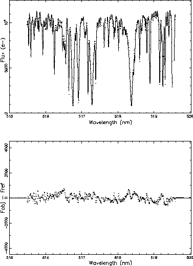
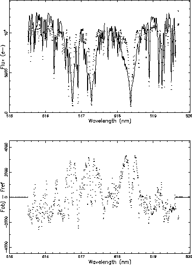
Then, the variance is calculated for each order. Figure 4 shows the fit between HD 41597 and HD 40460 (stars with similar parameters) and Figure 5 shows the fit between HD 41597 and HD 4628 (stars with different parameters).
 |
 |
Now comes the question of properly
combining the information contained in the different orders. This is not a trivial question.
First, there is a large variation of the S/N from the blue to the red orders.
Second the spectral information contained in each order is unequal.
The first problem is solved by weighting the variance obtained on each order by the the inverse of its mean flux. The degree of ressemblance between the target and the reference star is characterized by the expression :

with :

where :
K is the set of orders kept in the final result(see the next paragraph),
nb the number of orders
contained in K and <Fk> the mean flux of the target star for each order.
This expression is in practice equivalent to a reduced ![]() .
.
The second problem is the fact that some orders include strong lines of various
elements, whereas some others are almost free of lines. For example, order 119 including
the Mg I triplet appears to be one of the most significant orders for every star. Orders
94 and 127 containing ![]() and
and ![]() are very useful for effective
temperature determinations. Howewer its worth noticing that all orders depend on the
three parameters, which can not be estimated independently. The relative relevance of the
different orders has been studied. In order to select the best orders for each target.
The rms deviation of the fluxes, with respect to the mean flux, caused by
spectral lines plus noise, is computed. The 15 orders for which the ratio of this global
modulation to pure noise modulation is the highest, are kept.
This set of orders changes from one
target star to another, but the orders 127, 119 and 94 (including respectively
are very useful for effective
temperature determinations. Howewer its worth noticing that all orders depend on the
three parameters, which can not be estimated independently. The relative relevance of the
different orders has been studied. In order to select the best orders for each target.
The rms deviation of the fluxes, with respect to the mean flux, caused by
spectral lines plus noise, is computed. The 15 orders for which the ratio of this global
modulation to pure noise modulation is the highest, are kept.
This set of orders changes from one
target star to another, but the orders 127, 119 and 94 (including respectively ![]() ,the Mg I triplet and
,the Mg I triplet and ![]() ) are selected in almost every set.
The number of 15 has been chosen after
a number of ``try and see'' experiments over various S/N.
A larger number of orders introduce noise
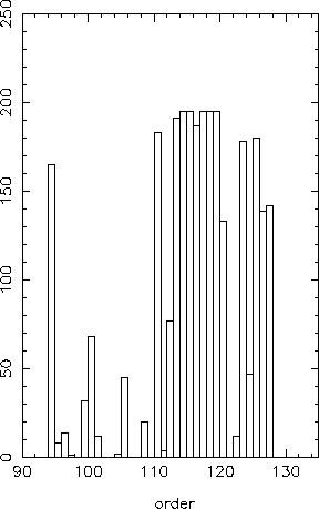
instead of information. Figure 6 shows the relative relevance of each order.
) are selected in almost every set.
The number of 15 has been chosen after
a number of ``try and see'' experiments over various S/N.
A larger number of orders introduce noise
instead of information. Figure 6 shows the relative relevance of each order.
 |
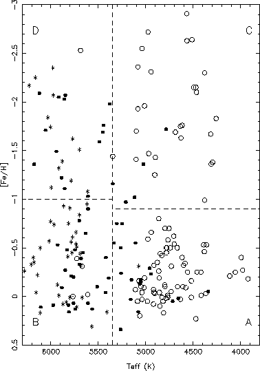
For a given target star, the comparison is performed with the 211 reference stars of the library.
The 10 reference stars showing the lowest reduced ![]() are selected.
The solution is given by the weighted mean of the parameters of the reference stars
whose reduced
are selected.
The solution is given by the weighted mean of the parameters of the reference stars
whose reduced ![]() is lower than 1.11 times the lowest one.
The upper limit of
is lower than 1.11 times the lowest one.
The upper limit of ![]() has been
empirically defined during the phase of test
(see Sect. 6) and is valuable only for target
stars with
has been
empirically defined during the phase of test
(see Sect. 6) and is valuable only for target
stars with ![]() . For smaller S/N the
limit is decreasing (i.e.
. For smaller S/N the
limit is decreasing (i.e. ![]() for S/N = 10).
for S/N = 10).
 |